Data Processing Pipeline
Preprocessing
A set of command line tools for data preprocessing steps is described in this section, which include data format conversion, data correction and brain extraction.
DICOM to NIFTI Conversion
For saving space of data store, the nii.gz format was used throughout the whole pipeline. Firstly, we use the dcm2nii (by Chris Rorden, https://www.nitrc.org/projects/dcm2nii) to convert the data into a single 3/4D .nii.gz volume-series file, plus bval and bvec files. The format of bval file is
0 1500 1500 ... 1500
and the format of bvec file is
0  0.99944484233856   0.00215385644697   0.00269041745923 ...
0  -0.0053533311002   0.99836695194244   0.60518479347229 ...
0  0.03288444131613  -0.05708565562963   -0.79608047008514 ...
where the 0 in the first column indicates the b0 images in the scan and certainly the software also supports multi-b0 images. Since the DICOM formats from different scanner might be different, this function is not always able to successfully extract the bvec/bval files. If you encounter such a problem, please get back to us <link> and give the link of your data if it has big size beyond the email capability.
$ ./dcm2nii -h
Compression will be faster with /usr/local/bin/pigz
Chris Rorden's dcm2niiX version 24Nov2014
usage: dcm2nii [options] <in_folder>
Options :

 -h   show help
 -f   filename (%c=comments %f=folder name %p=protocol %i ID of
      patient %n=name of patient %s=series, %t=time; default 'DTI')
 -o   output directory (omit to save to input folder)
 -z   gz compress images (y/n, default n)

Defaults file : /home/ccm/.dcm2nii.ini
Examples :
dcm2nii /Users/chris/dir
dcm2nii -o /users/cr/outdir/ -z y ~/dicomdir
dcm2nii -f mystudy%s ~/dicomdir
dcm2nii -o "~/dir with spaces/dir" ~/dicomdir
Example output filename: '/DTI.nii.gz'
Data correction
During the MRI scanning, many factors can cause distortions and misalignment.
The diffusion weighted imaging (DWI) volume series (as a 4D zipped NIFTI file)
are then corrected for the distortions induced by off-resonance field and the
misalignment caused by subject motion. The off-resonance effects are usually
caused by the eddy currents of switching the diffusion encoding gradients and
the susceptibility distribution of the imaged subjects, resulting in the deterioration
of images due to blurring, spatial distortion, local signal artifacts, etc. The
motion effects also cause image blurring and geometric misalignment [21]
[22].
To correct the distortions induced by susceptibility and eddy current when the data is acquired with different
phase-encode parameters, we include the correction mechanism using different
phase-encode information. We exported the functions of topup, applytopup, eddy and eddy_combine
from FSL [21]
[23]
[24],
compiled them on both Linux and Windows platforms, and packed the executable files
into DiffusionKit. The detailed usage information, please refer to the website of FSL (http://fsl.fmrib.ox.ac.uk/fsl/fslwiki/).
$ ./topup -h
Part of FSL (build 504)
topup

Usage:
topup --imain=<some 4D image> --datain=<text file> --config=<text file with parameters> --coutname=my_field


Compulsory arguments (You MUST set one or more of):
       --imain         name of 4D file with images
       --datain        name of text file with PE directions/times

Optional arguments (You may optionally specify one or more of):
       --out           base-name of output files (spline coefficients (Hz) and movement parameters)
       --fout          name of image file with field (Hz)
       --iout          name of 4D image file with unwarped images
       --logout        Name of log-file
       --warpres       (approximate) resolution (in mm) of warp basis for the different sub-sampling levels, default 10
       --subsamp       sub-sampling scheme, default 1
       --fwhm          FWHM (in mm) of gaussian smoothing kernel, default 8
       --config        Name of config file specifying command line arguments
       --miter         Max # of non-linear iterations, default 5
       --lambda        Weight of regularisation, default depending on --ssqlambda and --regmod switches. See user documetation.
       --ssqlambda     If set (=1), lambda is weighted by current ssq, default 1
       --regmod        Model for regularisation of warp-field [membrane_energy bending_energy], default bending_energy
       --estmov        Estimate movements if set, default 1 (true)
       --minmet        Minimisation method 0=Levenberg-Marquardt, 1=Scaled Conjugate Gradient, default 0 (LM)
       --splineorder   Order of spline, 2->Qadratic spline, 3->Cubic spline. Default=3
       --numprec       Precision for representing Hessian, double or float. Default double
       --interp        Image interpolation model, linear or spline. Default spline
       --scale         If set (=1), the images are individually scaled to a common mean, default 0 (false)
       --regrid        If set (=1), the calculations are done in a different grid, default 1 (true)
       -v,--verbose    Print diagonostic information while running
       -h,--help       display help info
$ ./eddy -h
Part of FSL (build 504)
eddy
Copyright(c) 2011, University of Oxford (Jesper Andersson)

Usage:
eddy --monsoon
Compulsory arguments (You MUST set one or more of):
       --imain File containing all the images to estimate distortions for
       --mask  Mask to indicate brain
       --index File containing indices for all volumes in --imain into --acqp and --topup
       --acqp  File containing acquisition parameters
       --bvecs File containing the b-vectors for all volumes in --imain
       --bvals File containing the b-values for all volumes in --imain
       --out   Basename for output

Optional arguments (You may optionally specify one or more of):
       --session       File containing session indices for all volumes in --imain
       --topup Base name for output files from topup
       --flm   First level EC model (linear/quadratic/cubic)
       --fwhm  FWHM for conditioning filter when estimating the parameters
       --niter Number of iterations (default 5)
       --resamp        Final resampling method (jac/lsr)
       --repol Detect and replace outlier slices
       -v,--verbose    switch on diagnostic messages
       -h,--help       display this message
Unfortunately, most clinical acquisitions do not currently meet the requirement
(two or more acquisitions where the parameters are different so that the mapping
fields for distortion correction are different.) of topup. To handle this issue,
we implemented a function called bneddy to correct eddy-current induced distortion
and head movements efficiently. bneddy applies rigid and affine registrations to
amend the distortions and misalignment.
$ ./bneddy -h
bneddy: Eddy Currents and Head Motion Correction.
(Mar 10 2016, 16:20:52)

   -i                Input file, 4D .nii.gz file.
   -o                Prefix for output file, and it will also output the log file as Prefix.txt which will be called by bnrotate_bvec.
   -ref     0        Reference image.
   -omp     2        Max number of threads
Skull Stripping (Brain Extraction)
This module is to strip the brain skull and extract the brain tissue, including gray matter, white matter, cerebrospinal fluid (CSF) and cerebellum. It largely benefits the following processing and analysis, offering better registration/alignment results and reducing computational time by excluding non-brain tissue. Therefore, although this step is not compulsory, we strongly recommend enforcing it. This module is adapted from the FSL/BET functions (http://fsl.fmrib.ox.ac.uk/fsl/fslwiki/BET) for its excellent efficacy and efficiency.
$ ./bet2 -h
Part of FSL (build 504)
BET (Brain Extraction Tool) v2.1 - FMRIB Analysis Group, Oxford
Usage:
bet2 <input_fileroot> <output_fileroot> [options]
Optional arguments (You may optionally specify one or more of):
       -o,--outline    generate brain surface outline overlaid onto original image
       -m,--mask <m>   generate binary brain mask
       -s,--skull      generate approximate skull image
       -n,--nooutput   don't generate segmented brain image output
       -f <f>          fractional intensity threshold (0->1); default=0.5; smaller values give larger brain outline estimates
       -g <g>          vertical gradient in fractional intensity threshold (-1->1); default=0; positive values give larger brain outline at bottom, smaller at top
       -r,--radius <r> head radius (mm not voxels); initial surface sphere is set to half of this
       -w,--smooth <r> smoothness factor; default=1; values smaller than 1 produce more detailed brain surface, values larger than one produce smoother, less detailed surface
       -c <x y z>      centre-of-gravity (voxels not mm) of initial mesh surface.
       -t,--threshold  -apply thresholding to segmented brain image and mask
       -e,--mesh       generates brain surface as mesh in vtk format
       -v,--verbose    switch on diagnostic messages
       -h,--help       displays this help, then exits
Reconstruction of the diffusion model
The reconstruction for diffusion model within pixels is one of the key topics in diffusion MRI research and it is also one of key modules of the software. At the current stage, we have integrated three modeling methods: one is the traditional Gaussian model (commonly known as DTI, diffusion tensor imaging), and the other two are for high angular resolution diffusion imaging (HARDI). For more detailed information please refer to our review paper [11] and [13] .
DTI Reconstruction
The classical diffusion gradient sequence used in dMRI is the pulsed gradient spin-echo (PGSE) sequence proposed by Stejskal and Tanner. This sequence has 90o and 180o gradient pulses with duration time δ and separation time Δ. To eliminate the dependence of spin density, we need at least two measurements of diffusion weighted imaging (DWI) signals, i.e. S(b) with the diffusion weighting factor b in Eq. (1) introduced by Le Bihan etc, and S(0) with b = 0 which is the baseline signal without any gradient.
$$ \begin{equation}\tag{1} b=\gamma^2 \delta^2 (\Delta-\frac{\delta}{3}){||\bf{G}||}^2 \end{equation} $$In the b-value in Eq. (1), $\gamma$ is the proton gyromagnetic ratio, $\bf{G}=||\bf{G}||\bf{u}$ is the diffusion sensitizing gradient pulse with norm $||{\bf G}||$ and direction ${\bf u}$. $\tau=\Delta-\frac{1}{3}\delta$ is normally used to describe the effective diffusion time. Using the PGSE sequence with S(b), the diffusion weighted signal attenuation E(b) is given by Stejskal-Tanner equation,
$$ \begin{equation}\tag{2} E(b)=\frac{S({b})}{S(0)}=\exp(-{b}D) \end{equation} $$where D is known as the apparent diffusion coefficient (ADC) which reflects the property of surrounding tissues. Note that in general ADC D is also dependent on G in a complex way. However, free diffusion in DTI assumes D is only dependent on the direction of G, i.e. . The early works in dMRI reported that ADC D is dependent on gradient direction u and used two or three DWI images in different directions to detect the properties of tissues. Then Basser et al. introduced diffusion tensor [12] to represent ADC as $D(\bf{u}) = {\bf u^{T}}{\bf D}\bf{u}$, where ${\bf D}$ is called as the diffusion tensor, which is a 3 × 3 symmetric positive definite matrix independent of ${\bf u}$. This method is called as diffusion tensor imaging (DTI) and is the most common method nowadays in dMRI technique. In DTI, the signal E(b) is represented as
$$ \begin{equation}\tag{3} E(b)=\exp(-b{\bf u^{T}}{\bf D}\bf{u}) \end{equation} $$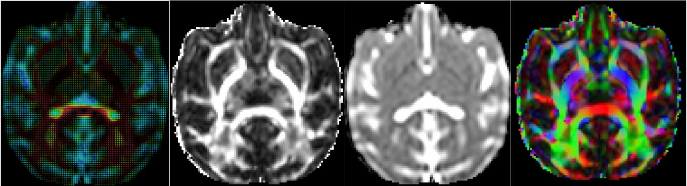
Figure 4. Tensor field and the scalar maps estimated from a monkey data with b = 1500s/mm2.
The diffusion tensor D can be estimated from measured diffusion signal samples through a simple least square method or weighted least square method [12], or more complex methods that consider positive definite constraint or Rician noise. If single b-value is used, the optimal b-value for tensor estimation was reported to in the range of (0.7~1.5)x$10^{3} s/mm^2$, and normally about twenty DWI images are used in DTI in clinical study. ome useful indices can be obtained from tensor D. The most important three indices are fractional anisotropy (FA), mean diffusivity (MD) and relative anisotropy (RA) defined as
$$ \begin{equation}\tag{4} {\rm{FA}}=\frac{\sqrt{3}||{\rm{D}}-\frac{1}{3} \rm{trace} ({\rm{D}}) I ||}{\sqrt{2}||{\rm{D}}||} =\sqrt{\frac{3}{2}}\sqrt{\frac{(\lambda_1-\bar{\lambda})^2+(\lambda_2-\bar{\lambda})^2+(\lambda_3-\bar{ \lambda})^2}{\lambda_{1}^{2}+\lambda_{2}^{2}+\lambda_{3}^{2}}} \end{equation} $$$$ \begin{equation}\tag{5} {\rm{MD}}=\bar{\lambda}=\frac{1}{3} \rm{trace} ({\rm{D}})=\frac{\lambda_1+\lambda_2+\lambda_3}{3} \end{equation} $$$$ \begin{equation}\tag{6} {\rm{RA}}=\sqrt{\frac{(\lambda_1-\bar{\lambda})^2+(\lambda_2-\bar{\lambda})^2+(\lambda_3-\bar{\lambda})^2}{3\bar{\lambda}}} \end{equation} $$where, are the three eigenvalues of D and is the mean eigenvalue. MD and FA have been used in many clinical applications. For example, MD is known to be useful in stroke study. For more detailed information please refer to our review paper [13].
$ ./bndti_estimate -h
bndti_estimate: Diffusion Tensors Estimation.
DiffusionKit (v1.3), http://diffusion.brainnetome.org/.
(Jun 24 2016, 09:40:15)

general arguments
   -d                    Input DWI Data, in NIFTI/Analyze format (4D)
   -g                    Gradients direction file
   -b                    b value file
   -m                    Brain mask : filein mask | OPTIONAL
   -o          dti       Result DTI : fileout prefix; 'dti' by default
   -tensor     0         Save tensor : 0 - No; 1 - Yes; (Default: 0)
   -eig        0         Save eigenvalues and eigenvectors : 0 - No; 1 - Yes; (Default: 0)
SPFI Reconstruction
It was proposed that the SPFI method has more powerful capability to identify the tangling fibers [8]. In SPFI [8], the diffusion signal is represented by spherical polar Fourier (SPF) basis functions in Eq. 7.
$$\begin{equation} \tag{7} E(q)=\sum_{n=0}^{N}\sum_{l=0}^{L}\sum_{m=-l}^{l} a_{lmn}R_{n}(||q||)Y_{l}^{m}(u) \end{equation}$$The SPF basis denoted by $R_{n}(||q||)Y_{l}^{m}(u)$ is a 3D orthonormal basis with spherical harmonics in the spherical portion and the Gaussian-Laguerre function in the radial portion. Furthermore, Cheng and his colleagues proposed a uniform analytical solution to transform the coefficients $a_{lmn}$ of $E(q)$ to the coefficients $c_{lm}^{\Phi_w}$ of ODF (orientation distribution function) represented by the spherical harmonics basis, as in Eq. 8.
$$\begin{equation} \tag{8} \Phi_w(r)=\sum_{l=0}^{L}\sum_{m=-l}^{l}c_{lm}^{\Phi_w}Y_{l}^{m}(r) \end{equation}$$It is a model-free, regularized, fast and robust reconstruction method which can be performed with single-shell or multiple-shell HARDI data to estimate the ODF proposed by Wedeen et al. [14]. The implementation of analytical SPFI includes two independent steps. The first estimates the coefficients of $E(q)$ with least squares, and the second transforms the coefficients of $E(q)$ to the coefficients of ODF.
$ ./bnhardi_ODF_estimate -h
bnhardi_ODF_estimate: Orientation Distribution Function Estimation (SPFI method).
DiffusionKit (v1.3), http://diffusion.brainnetome.org/.
(Jun 24 2016, 09:40:28)
   -d                        Input DWI data (4D NIfTI file).
   -b                        Text file for b-values.
   -g                        Text file for grad directions.
   -m                        Input brain mask.
   -o                        Output prefix for EAP profile and ODF file.
   -scale          -1        The scale parameter of Spherical Polar Fourier Basis. The default is calculated by the program.
   -tau            0.02533   The diffusion time of DWI data.
   -outGFA         false     Whether output generalized FA. True means Yes.
   -rdis           0.015     The radius value for EAP profile.
   -sh             4         Order of spherical basis
   -ra             1         Order of radial basis
   -lambda_sh      0         Regularization parameter for spherical basis
   -lambda_ra      0         Regularization parameter for radial basis
CSD Reconstruction
The CSD method was proposed by Tournier et al. [9], which expresses the diffusion signal as in Eq. 9,
$$\begin{equation} \tag{9} S(\theta,\Phi) = F(\theta,\Phi)\otimes R(\theta) \end{equation}$$where $F(\theta,\Phi)$ is called the fiber orientation density function (fODF), which needs to be estimated, and $R(\theta)$ is the response function, which is the typical signal generated from one fiber. The response function can be directly estimated from diffusion weighted image (DWI) data by measuring the diffusion profile in the voxels with the highest fractional anisotropy values, indicating that a single coherently oriented fiber population is contained in these voxels. When the response function is obtained, we can utilize the deconvolution of $R(\theta)$ from $F(\theta,\Phi)$ to estimate the fiber ODF. The computation of the fiber ODF was carried out using the software MRtrix (J-D Tournier, Brain Research Institute, Melbourne, Australia, http://www.brain.org.au/software/). We thank Dr. Jacques-Donald Tournier for sharing MATLAB code of the CSD method, which inspired an efficient C/C++ implementation.
$ ./bnhardi_FOD_estimate -h
bnhardi_FOD_estimate: Constraind Spherical Deconvolution (CSD) based HARDI reconstruciton.
DiffusionKit (v1.2), http://diffusion.brainnetome.org/.
(Jul 15 2015, 11:50:20)
general arguments
   -d                            Input DWI Data, in NIFTI/Analyze format (4D)
   -g                            Gradients direction file
   -b                            b value file
   -m                            Brain mask : filein mask | OPTIONAL
   -outFA        1               Whether to output the FA of DTI
   -o                            Result CSD Estimate (.nii.gz)
   -lmax         8               6/8/10, Max order of the adopted harmonical base
   -fa           [0.75,0.95]     The FA thesshold considered as single fiber
   -erode        -1              The unit is voxel: Remove the garbage near the boundary of FA image,
                                 for better estimating response function
   -nIter        50              Max iteration number before aborting
   -lambda       1               The regularization weight for optimization
   -tau          0.1             The threshold on the FOD amplitude used to identify negative lobes
   -hr           300             300/1000/5000. The later get more acurate estimation while more
                                 time consuming, so use the first one unless your computer
                                 is powerful !
bnhardi_FOD_estimate: Constraind Spherical Deconvolution (CSD) based HARDI reconstruciton.
DiffusionKit (v1.3), http://diffusion.brainnetome.org/.
(Jun 24 2016, 09:40:29)
general arguments
   -d                           Input DWI Data, in NIFTI/Analyze format (4D)
   -g                           Gradients direction file
   -b                           b value file
   -m                           Brain mask : filein mask | OPTIONAL
   -outFA          1            Whether to output the FA of DTI
   -o                           Result CSD Estimate (.nii.gz)
   -lmax           8            6/8/10, Max order of the adopted harmonical base
   -fa             [0.75,0.95]  The FA thesshold considered as single fiber
   -erode          -1           The unit is voxel: Remove the garbage near the boundary of FA image, for better estimating response function
   -nIter          50           Max iteration number before aborting
   -lambda         1            The regularization weight for optimization
   -tau            0.1          The threshold on the FOD amplitude used to identify negative lobes
   -hr             300          300/1000/5000. The later get more acurate estimation while more time consuming, so use the first one unless your computer is powerful !
   -omp            2            Max number of threads
Fiber tracking and attributes extraction
Fiber tracking is a critical way to construct the anatomical connectivity matrix. For the tracking based on tensors from DTI, an intuitive way is to link the neighboring voxels following their main directions (e.g. V1 in the eigenvector of the DTI) given a set of some stop criteria, such as maximum bending angle of the curve and minimum FA value, which is to ensure the target voxel is indeed white matter microstructure. This is the so called deterministic streamline tractography [15], as illustrated in Figure 5.
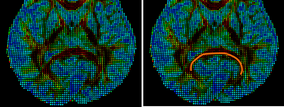
Figure 5. Illustration for deterministic streamline tractography.
$ ./bndti_tracking -h
bndti_tracking: DTI Deterministic Fibertracking.
DiffusionKit (v1.3), http://diffusion.brainnetome.org/.
(Jun 24 2016, 09:40:29)
   -d                   Input DTI data.
   -m                   Mask Image.
   -s                   Seeds Image.
   -fa                  FA Image.
   -invert     0        Invert x: 1; Invert y: 2; Invert z: 3.
   -swap       0        Swap x/y: 1; Swap x/z: 2; Swap y/z: 3.
   -ft         0.1      FA Threshold.
   -at         45       Angular Threshold.
   -sl         0.5      Step Length (Voxel).
   -min        10       Threshold the fiber (mm). (remove fibers shorter than the number)
   -max        5000     Upper-threshold the fiber (mm). (remove fibers longer than the number)
   -o                   Output Fibers Filename (.trk file).
The tracking module in the software for HARDI estimation is similar to the streamline method as described above. It should be kept in mind that, for HARDI estimation, usually there are more than one main direction (which is what we desired since it possibly identifies tangling fibers), so we should consider these kissing/branching cases. Meanwhile, since there is no explicit dominant directions for each voxel, searching algorithm should be applied to locate the main directions. The searching should run for each voxel, so it is not as fast as the traditional DTI tracking.
$ ./bnhardi_tracking -h
bnhardi_tracking: HARDI Deterministic Fibertracking.
DiffusionKit (v1.3), http://diffusion.brainnetome.org/.
(Jun 24 2016, 09:40:28)
   -d                        HARDI spherical harmonic image.
   -fa                       FA image.
   -m                        Mask image.
   -s                        Seeds image.
   -sl           0.5         Step length (Voxel): float.
   -ft           0.1         FA threshold: float.
   -at           60          Angle threshold: float.
   -min          10          Threshold the fiber (mm). (remove fibers shorter than the number)
   -max          5000        Upper-threshold the fiber (mm). (remove fibers longer than the number)
   -invert       0           Invert x: 1; Invert y: 2; Invert z: 3.
   -swap         0           Swap x/y: 1; Swap x/z: 2; Swap y/z: 3.
   -threshold    0.25        Threshold for the peaks of ODF.
   -omp          1           Max number of threads.
   -o                        Tract file (.trk file).
Visualization for various images
The software provides a variety of entries for visualizing different data types, including 3D/4D image, Tensor/ODF/FOD image and white mater fibers. The views of different data could be superimposed for a precise anatomical localization. It should be noted that, if one uses the GUI, these view functions could be called in each processing steps for inspecting the results.
Figure 6. Illustrations for the capability of the software to show many types of images.
$ ./bnviewer -h
This program is the GUI frontend that displays and performs data reconstruction and fiber tracking on diffusion MR images, which have been developed by the teams of Brainnetome Center, CASIA.
basic usage:
  bnviewer [[-volume] DTI_FA.nii.gz]
           [-roi ROI/roi_cc_top.nii.gz]
           [-fiber ROI/roi_cc_top.trk]
           [-tensor DTI.nii.gz]/[-odf HARDI.nii.gz]

options:
  -help                  show this help
  -volume  .nii.gz       set input background data
  -roi     .nii.gz       set input ROI data
  -fiber   .trk          set input fiber data
  -tensor  .nii.gz       set input DTI data (conflict with -odf args)
  -odf     .nii.gz       set input ODF/FOD data (conflict with -tensor args)
Several other useful tools
Image registration
This module is implemented by NiftyReg, which is an open-source software
for efficient medical image registration. It has been mainly developed by
members of the Translational Imaging Group with the Centre for Medical
Image Computing at University College London, UK [10].
In our software, the registration module is customized to auto-configure
the parameter settings for different image modalities, e.g., two DWI
images (for eddy current correction in current version), standard space and T1
space (for mapping ROIs to the individual space), DWI space and
standard space (for statistical comparisons across subjects). This
module contains several commands reg_aladin is the command for
rigid and affine registration which is based on a block-matching approach and
a Trimmed Least Square (TLS) scheme [18]
[19]. reg_f3d is the command to perform
non-linear registration which is based on the Free-From Deformation presented
by Rueckert et al. [20]. reg_resample is
been embedded in the package. It uses the output of reg_aladin and
reg_f3d to apply transformation, generate deformation fields or
Jacobian map images for example.
$ ./reg_aladin -h
Block Matching algorithm for global registration.
Based on Ourselin et al., "Reconstructing a 3D structure from serial histological sections", Image and Vision Computing, 2001

Usage: reg_aladin -ref <filename> -flo <filename> [OPTIONS].
       -ref <filename> Reference image filename (also called Target or Fixed) (mandatory)
       -flo <filename> Floating image filename (also called Source or moving) (mandatory)

OPTIONS
       -noSym                  The symmetric version of the algorithm is used by default. Use this flag to disable it.
       -rigOnly                To perform a rigid registration only. (Rigid+affine by default)
       -affDirect              Directly optimize 12 DoF affine. (Default is rigid initially then affine)
       -aff <filename>         Filename which contains the output affine transformation. [outputAffine.txt]
       -inaff <filename>       Filename which contains an input affine transformation. (Affine*Reference=Floating) [none]
       -rmask <filename>       Filename of a mask image in the reference space.
       -fmask <filename>       Filename of a mask image in the floating space. (Only used when symmetric turned on)
       -res <filename>         Filename of the resampled image. [outputResult.nii]
       -maxit <int>            Maximal number of iterations of the trimmed least square approach to perform per level. [5]
       -ln <int>               Number of levels to use to generate the pyramids for the coarse-to-fine approach. [3]
       -lp <int>               Number of levels to use to run the registration once the pyramids have been created. [ln]
       -smooR <float>          Standard deviation in mm (voxel if negative) of the Gaussian kernel used to smooth the Reference image. [0]
       -smooF <float>          Standard deviation in mm (voxel if negative) of the Gaussian kernel used to smooth the Floating image. [0]
       -refLowThr <float>      Lower threshold value applied to the reference image. [0]
       -refUpThr <float>       Upper threshold value applied to the reference image. [0]
       -floLowThr <float>      Lower threshold value applied to the floating image. [0]
       -floUpThr <float>       Upper threshold value applied to the floating image. [0]
       -nac                    Use the nifti header origin to initialise the transformation. (Image centres are used by default)
       -cog                    Use the input masks centre of mass to initialise the transformation. (Image centres are used by default)
       -interp                 Interpolation order to use internally to warp the floating image.
       -iso                    Make floating and reference images isotropic if required.
       -pv <int>               Percentage of blocks to use in the optimisation scheme. [50]
       -pi <int>               Percentage of blocks to consider as inlier in the optimisation scheme. [50]
       -speeeeed               Go faster
       -omp <int>              Number of thread to use with OpenMP. [4]
       -voff                   Turns verbose off [on]
$ ./reg_f3d -h
Fast Free-Form Deformation algorithm for non-rigid registration.
Based on Modat et al., "Fast Free-Form Deformation using graphics processing units", CMPB, 2010

Usage: reg_f3d -ref <filename> -flo <filename> [OPTIONS].
       -ref <filename> Filename of the reference image (mandatory)
       -flo <filename> Filename of the floating image (mandatory)

OPTIONS
Initial transformation options (One option will be considered):
       -aff <filename>         Filename which contains an affine transformation (Affine*Reference=Floating)
       -incpp <filename>       Filename ofloatf control point grid input

Output options:
       -cpp <filename>         Filename of control point grid [outputCPP.nii]
       -res <filename>         Filename of the resampled image [outputResult.nii]

Input image options:
       -rmask <filename>               Filename of a mask image in the reference space
       -smooR <float>                  Smooth the reference image using the specified sigma (mm) [0]
       -smooF <float>                  Smooth the floating image using the specified sigma (mm) [0]
       --rLwTh <float>                 Lower threshold to apply to the reference image intensities [none]. Identical value for every timepoint.*
       --rUpTh <float>                 Upper threshold to apply to the reference image intensities [none]. Identical value for every timepoint.*
       --fLwTh <float>                 Lower threshold to apply to the floating image intensities [none]. Identical value for every timepoint.*
       --fUpTh <float>                 Upper threshold to apply to the floating image intensities [none]. Identical value for every timepoint.*
       -rLwTh <timepoint> <float>      Lower threshold to apply to the reference image intensities [none]*
       -rUpTh <timepoint> <float>      Upper threshold to apply to the reference image intensities [none]*
       -fLwTh <timepoint> <float>      Lower threshold to apply to the floating image intensities [none]*
       -fUpTh <timepoint> <float>      Upper threshold to apply to the floating image intensities [none]*

Spline options:
       -sx <float>             Final grid spacing along the x axis in mm (in voxel if negative value) [5 voxels]
       -sy <float>             Final grid spacing along the y axis in mm (in voxel if negative value) [sx value]
       -sz <float>             Final grid spacing along the z axis in mm (in voxel if negative value) [sx value]

Regularisation options:
       -be <float>             Weight of the bending energy penalty term [0.005]
       -le <float> <float>     Weights of linear elasticity penalty term [0.0 0.0]
       -l2 <float>             Weights of L2 norm displacement penalty term [0.0]
       -jl <float>             Weight of log of the Jacobian determinant penalty term [0.0]
       -noAppJL                To not approximate the JL value only at the control point position

Measure of similarity options:
NMI with 64 bins is used expect if specified otherwise
       --nmi                   NMI. Used NMI even when one or several other measures are specified.
       --rbn <int>             NMI. Number of bin to use for the reference image histogram. Identical value for every timepoint.
       --fbn <int>             NMI. Number of bin to use for the floating image histogram. Identical value for every timepoint.
       -rbn <tp> <int>         NMI. Number of bin to use for the reference image histogram for the specified time point.
       -rbn <tp> <int>         NMI. Number of bin to use for the floating image histogram for the specified time point.
       --lncc <float>          LNCC. Standard deviation of the Gaussian kernel. Identical value for every timepoint
       -lncc <tp> <float>      LNCC. Standard deviation of the Gaussian kernel for the specified timepoint
       --ssd                   SSD. Used for all time points
       -ssd <tp>               SSD. Used for the specified timepoint
       --kld                   KLD. Used for all time points
       -kld <tp>               KLD. Used for the specified timepoint
       -amc                    To use the additive NMI for multichannel data (bivariate NMI by default)

Optimisation options:
       -maxit <int>            Maximal number of iteration per level [300]
       -ln <int>               Number of level to perform [3]
       -lp <int>               Only perform the first levels [ln]
       -nopy                   Do not use a pyramidal approach
       -noConj                 To not use the conjuage gradient optimisation but a simple gradient ascent
       -pert <int>             To add perturbation step(s) after each optimisation scheme

F3D2 options:
       -vel                    Use a velocity field integration to generate the deformation
       -fmask <filename>       Filename of a mask image in the floating space

OpenMP-related options:
       -omp <int>              Number of thread to use with OpenMP. [4]

Other options:
       -smoothGrad <float>     To smooth the metric derivative (in mm) [0]
       -pad <float>            Padding value [nan]
       -voff                   To turn verbose off
$ ./reg_resample -h
Usage: reg_resample -ref <filename> -flo <filename> [OPTIONS].
       -ref <filename>      Filename of the reference image (mandatory)
       -flo <filename>      Filename of the floating image (mandatory)

OPTIONS
       -trans <filename>    Filename of the file containing the transformation parametrisation (from reg_aladin, reg_f3d or reg_transform)
       -res <filename>      Filename of the resampled image [none]
       -blank <filename>    Filename of the resampled blank grid [none]
       -inter <int>         Interpolation order (0, 1, 3, 4)[3] (0=NN, 1=LIN; 3=CUB, 4=SINC)
       -pad <int>           Interpolation padding value [0]
       -tensor              The last six timepoints of the floating image are considered to be tensor order as XX, XY, YY, XZ, YZ, ZZ [off]
       -psf                 Perform the resampling in two steps to resample an image to a lower resolution [off]
       -voff                Turns verbose off [on]
Need further help?
Check the website http://cmictig.cs.ucl.ac.uk/wiki/index.php/NiftyReg.
Image calculation and ROI generation
The module bncalc provides simple image calculations,
such as add/minus/multiply/divide operations.
Meanwhile, it can also generate user-defined ROIs given
the origin and radius in a user-specified image space.
$ ./bncalc -h
DiffusionKit (v1.3), http://diffusion.brainnetome.org/.
This funciton provide basic process for the input data (NIFTI/Analyze format)
Usage of bncalc:
   -i       image         The original file you want to manage.
   -add     image/value   Add to the data from the last step.
   -sub     image/value   Subtract data from the last step.
   -mul     image/value   Multiply the data from the last step.
   -div     image/value   Divide the data from the last step.
   -roi     x,y,z,r       Generate a ROI centered at [x,y,z](MNI mm) with radius r, in the input data space.
   -roi_rect  x1,x2,y1,y2,z1,z2  OR  i
                          Generate a cuboid ROI by specifying left-bottom
                          corner [x1,y1,z1] and right-up corner [x2,y2,z2].
                          If only one integer is specified, we assume you
                          want to get the i-the volume along the 4th dimension (from 0).
   -mask    image         Mask the data from last step by this input one.
                          If this input is a binary, then it is the same as
                          -mul, otherwise it keep the voxels from the last step
                          when the new input is nonzero.
   -bin     value         set 1 if >value, otherwise 0.
   -uthr    value         Set voxel=0 when it>value.
   -dthr    value         Set voxel=0 when it<value.
   -o       image         output a NIFTI (.nii.gz) file
Fiber manipulation
After obtaining a large bundle of white matter fibers, you may want to prune
the fibers that go through specified locations (ROIs). Here, we provide
several tools to manipulate the fiber bundles. bnfiber_prune, to
split fiber bundles based on given ROIs.
$ ./bnfiber_prune
bnfiber_prune: Prune fiber bundles based on given ROIs.
DiffusionKit (v1.3), http://diffusion.brainnetome.org/.
(Jun 24 2016, 09:40:29)
   -fiber          Tract file (.trk file)
   -and            AND ROI file: ro1.nii.gz,roi2.nii.gz
   -or             OR ROI file: roi1.nii.gz,roi2.nii.gz
   -not            NOT ROI file: ro1.nii.gz,roi2.nii.gz
   -o              Output Tract file (.trk file).
bnfiber_end, to cut the fiber bundles given start/stop ROIs, which is useful
to get the exact connections between two ROIs in constructing connectivity matrix.
$ ./bnfiber_end -h
bnfiber_end: Extract fibers which end in the two given rois.
DiffusionKit (v1.3), http://diffusion.brainnetome.org/.
(Jun 24 2016, 09:40:29)
   -fiber          Tract file (.trk file).
   -roi1           ROI1 file
   -roi2           ROI2 file
   -o              Output tract file (.trk file)
bnfiber_stats, to extract statistical properties of the fiber bundle, such
as mean FA/MD and fiber numbers.
$ ./bnfiber_stats -h
bnfiber_stats: Show fiber stats.
DiffusionKit (v1.3), http://diffusion.brainnetome.org/.
(Jun 24 2016, 09:40:33)
   -fiber          Input tract file (.trk file).
bnfiber_map, to compute the fiber density map which is used in track density imaging [16].
$ ./bnfiber_map -h
bnfiber_map: Calculate the fiber density.
DiffusionKit (v1.3), http://diffusion.brainnetome.org/.
(Jun 24 2016, 09:40:29)
   -fiber             Fiber file (.trk).
   -o                 Output file (NIfTI).
   -nor        1      Normalize fiber density: 1 (yes) or 0 (no).
bnmerge / bnsplit, to merge the 3D volumes to 4D or split 4D to 3D volumes.
$ ./bnmerge -h
bnmerge: Merge 3D NIfTI files  to 4D NIfTI file.
   This program is to merge 3D NIfTI files to 4D NIfTI file.
   Usage: bnmerge filein1 filein2 ... fileout
   options:     -h           : show this help
$ ./bnsplit -h
bnsplit: Split 4D volume to 3D volumes.
   This program splits 4D volume to 3D volumes.
   basic usage: split -i FILE_IN -o FILE_OUT prefix
   options:     -h           : show this help
                -v LEVEL     : the verbose level to LEVEL
bninfo, to display a short head information of the input image. Supported input image format includes NIFTI/DICOM.
$ ./bninfo -h
Show file header information.
DiffusionKit (v1.3), http://diffusion.brainnetome.org/.
Options:
  -h,--help           Print this help information
  -c,--is-canonical   Check XFORM and parse whether transform matrix is canoical